5: Fire Severity using Normalized Burn Index

library(sf)
library(stars)
library(tidyverse)
library(tmap)
library(rstac)
library(gdalcubes)

url <- "https://34c031f8-c9fd-4018-8c5a-4159cdff6b0d-cdn-endpoint.azureedge.net/-/media/calfire-website/what-we-do/fire-resource-assessment-program---frap/gis-data/april-2023/fire221gdb.zip?rev=9e3e1e5e61e242d5b2994d666d72a91a&hash=F424990CD64BB7C4CF01C6CE211C0A59"
download.file(url, "fire221.gdb.zip",  mode="wb")



unzip("fire221.gdb.zip")

fire_polys <- 
  read_sf("fire22_1.gdb", layer = "firep22_1") |> 
  filter(st_is_valid(Shape))

jtree <- 
  read_sf("/vsicurl/https://huggingface.co/datasets/cboettig/biodiversity/resolve/main/data/NPS.gdb") |> 
  filter(UNIT_NAME == "Joshua Tree National Park") |> 
  st_transform(st_crs(fire_polys))

fire_is_in_jtree <- st_intersects(fire_polys, jtree, sparse=FALSE)
fire_jtree <- fire_polys |> filter(fire_is_in_jtree)

Warning: Using one column matrices in `filter()` was deprecated in dplyr 1.1.0.
ℹ Please use one dimensional logical vectors instead.

tmap_mode("view")

tmap mode set to 'view'

tm_shape(jtree) + tm_polygons() + 
 tm_shape(fire_jtree) + tm_polygons("YEAR_")

Because burned vegetation presents a very different spectral pattern to normal vegetation, burn intensity can be measured by comparing the spectra in different bands. The greatest contrast between burned and health vegetation can be seen in the NIR and SWIR bands, as seen in this typical spectral response curve:

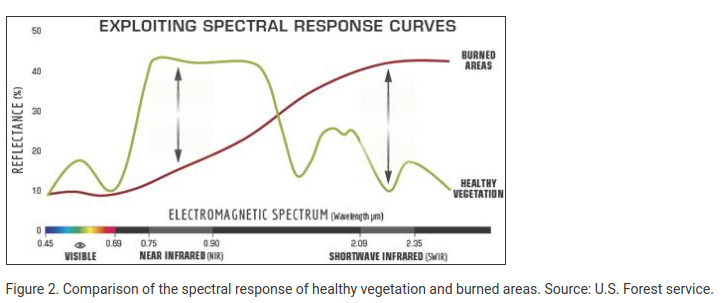
The normalized burn ratio (NBR) is defined as the ratio:

\[ NBR = \frac{NIR - SWIR}{NIR + SWIR}\]

Landsat example

Sentinel-2 Example

big_fire <- fire_jtree |> 
  filter(YEAR_ > "2015") |> 
  filter(Shape_Area == max(Shape_Area)) 


box <- big_fire |> st_transform(4326) |> st_bbox() 
alarm_date <- big_fire$ALARM_DATE

start_date <- as.character( alarm_date - days(5) )
end_date <- as.character( alarm_date + days(5) )

items <-  
  stac("https://planetarycomputer.microsoft.com/api/stac/v1")  |>
  stac_search(collections = "sentinel-2-l2a",
              datetime = paste(start_date, end_date, sep="/"),
              bbox = c(box))  |>
  post_request() |>
  items_sign(sign_planetary_computer())

col <- stac_image_collection(items$features, asset_names = c("B08", "B12", "SCL"))

cube <- cube_view(srs ="EPSG:4326",
                  extent = list(t0 = start_date, t1 = end_date,
                                left = box[1], right = box[3],
                                top = box[4], bottom = box[2]),
                  dx = 0.0001, dy = 0.0001, dt = "P1D")

mask <- image_mask("SCL", values=c(3, 8, 9)) # mask clouds and cloud shadows
data <-  raster_cube(col, cube, mask = mask)

nbr <- data |> 
  apply_pixel("(B08-B12)/(B08+B12)", "NBR") 

before_fire <- nbr |> slice_time("2022-05-25") 
after_fire <- nbr  |> slice_time("2022-05-30")

before_fire |> plot()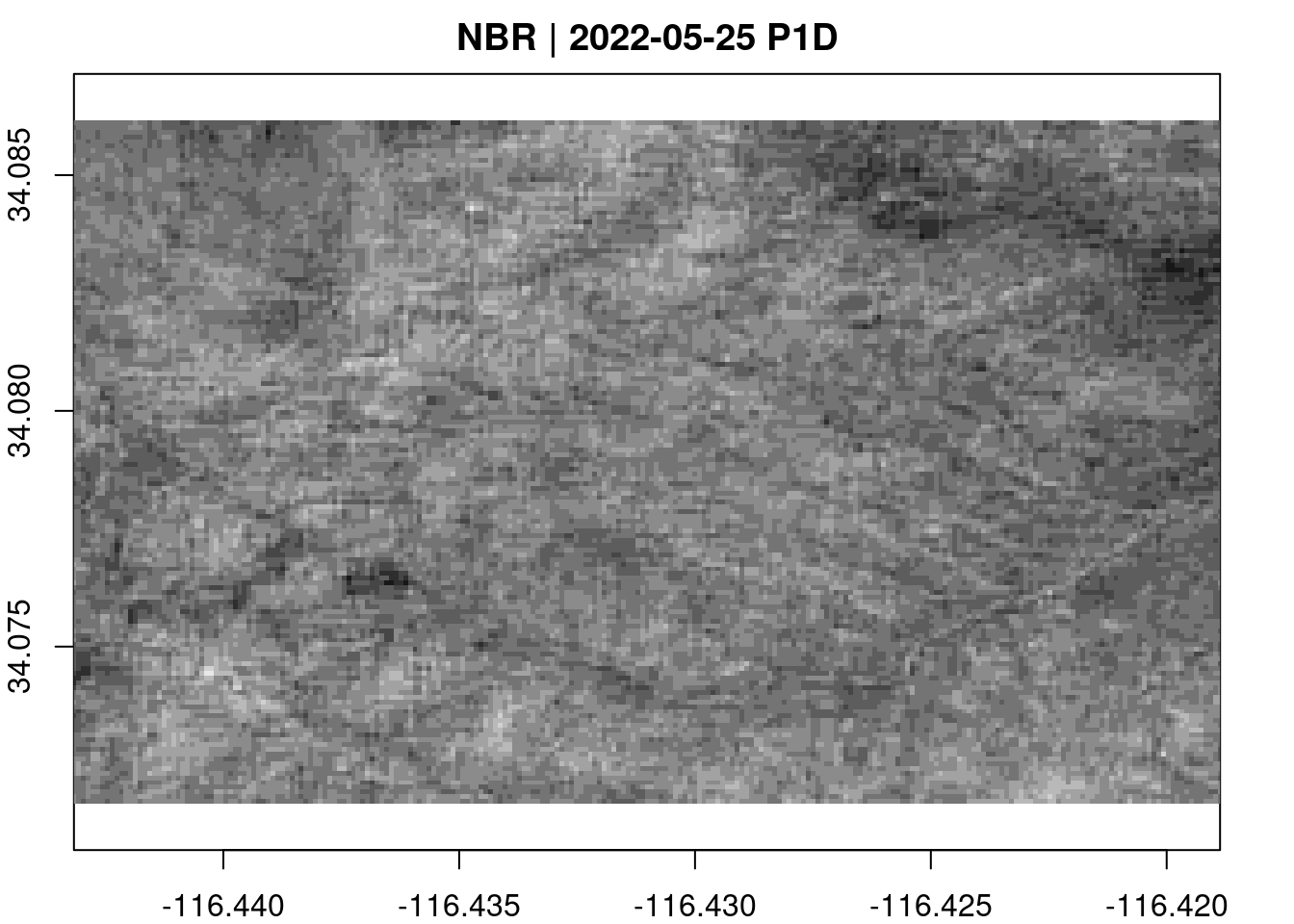

after_fire |> plot()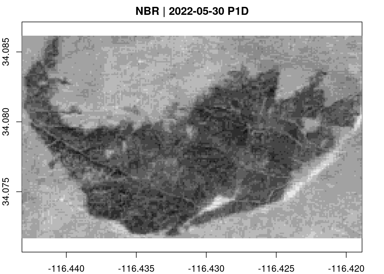

after_fire_stars <- after_fire |> st_as_stars()

Warning in CPL_read_gdal(as.character(x), as.character(options),
as.character(driver), : GDAL Message 1: The dataset has several variables that
could be identified as vector fields, but not all share the same primary
dimension. Consequently they will be ignored.

before_fire_stars <- before_fire |> st_as_stars()

Warning in CPL_read_gdal(as.character(x), as.character(options),
as.character(driver), : GDAL Message 1: The dataset has several variables that
could be identified as vector fields, but not all share the same primary
dimension. Consequently they will be ignored.

st_dimensions(before_fire_stars) <- st_dimensions(after_fire_stars)

dnbr <- before_fire_stars - after_fire_stars

tmap_mode("view")

tmap mode set to 'view'

tm_shape(dnbr) + tm_raster() +
tm_shape(big_fire) + tm_borders() 

[scale] tm_raster:() the data variable assigned to 'col' contains positive and negative values, so midpoint is set to 0. Set 'midpoint = NA' in 'fill.scale = tm_scale_intervals(<HERE>)' to use all visual values (e.g. colors)

with slider

We can use leaflet to create a slider bar. This is more verbose than tmap but very powerful. (Note that this example requires the GitHub)

library(leaflet.extras2)

Loading required package: leaflet

library(terra) # leaflet doesn't know about the stars package yet

terra 1.7.71

Attaching package: 'terra'

The following objects are masked from 'package:gdalcubes':

    animate, crop, size

The following object is masked from 'package:tidyr':

    extract

    Map <- leaflet() |> 
      addMapPane("right", zIndex = 0) |> 
      addMapPane("left",  zIndex = 0) |>
      addTiles(group = "base", layerId = "baseid1", options = pathOptions(pane = "right")) |> 
      addTiles(group = "base", layerId = "baseid2", options = pathOptions(pane = "left")) |> 
      addRasterImage(x = rast(after_fire_stars), options = leafletOptions(pane = "right"), group = "r1") |> 
      addRasterImage(x = rast(before_fire_stars), options = leafletOptions(pane = "left"), group = "r2") |> 
      addLayersControl(overlayGroups = c("r1", "r2")) |>  
      addSidebyside(layerId = "sidecontrols",
                    rightId = "baseid1",
                    leftId  = "baseid2")
    


Map