library(rstac)
library(gdalcubes)
library(stars)
library(tmap)
library(dplyr)
earthdatalogin::gdal_cloud_config()
earthdatalogin::with_gdalcubes()3: animations
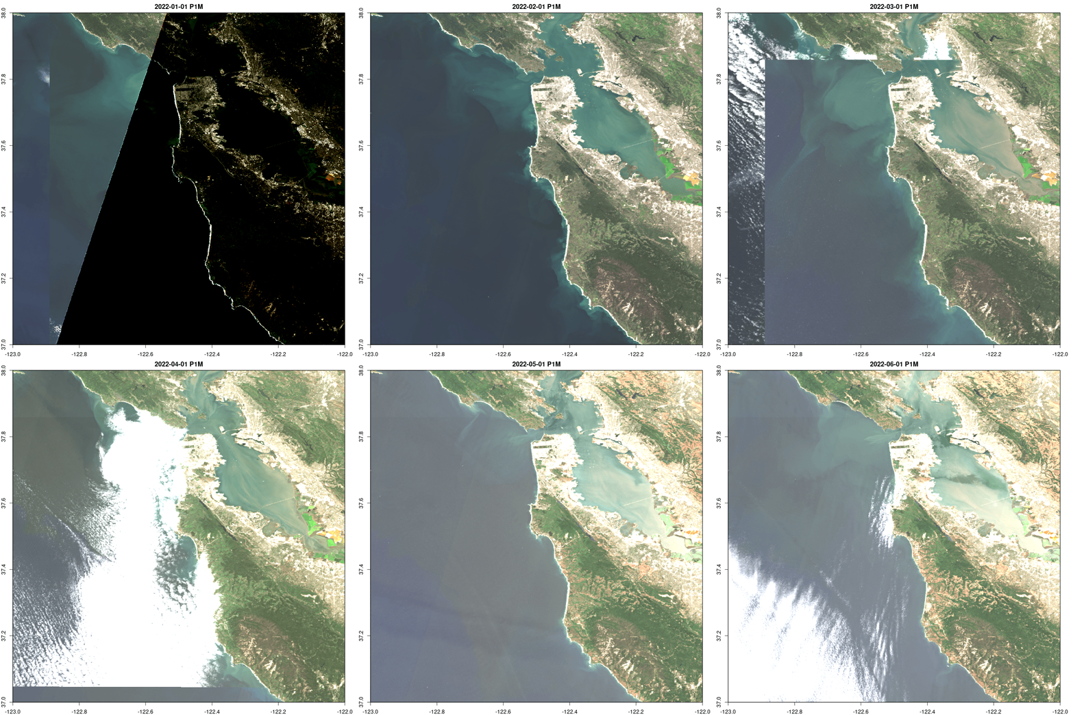
Following the same template, but we compute over a larger bounding box and generate an animation
box <- c(xmin=-123, ymin=37, xmax=-122, ymax=38)
start_date <- "2022-01-01"
end_date <- "2022-06-30"
items <-
  stac("https://planetarycomputer.microsoft.com/api/stac/v1") |>
  stac_search(collections = "sentinel-2-l2a",
              bbox = box,
              datetime = paste(start_date, end_date, sep="/"),
              limit = 1000) |>
  ext_query("eo:cloud_cover" < 20) |>
  post_request() |>
  items_sign(sign_planetary_computer())
Let’s do a true-color RGB image this time by combining data from Blue, Green, and Red bands:
col <- stac_image_collection(items$features, asset_names = c("B02", "B03", "B04", "SCL"))

cube <- cube_view(srs ="EPSG:4326",
                  extent = list(t0 = start_date, t1 = end_date,
                                left = box[1], right = box[3],
                                top = box[4], bottom = box[2]),
                  dx = 0.001, dy = 0.001, dt = "P1M")

data <-  raster_cube(col, cube)
ndvi <- data |>
select_bands(c("B02","B03", "B04")) |>
write_ncdf("visual.nc", overwrite=TRUE)While we could go directly from apply_pixel to animate, here we show how to stash a copy of the computed, rescaled and reprojected data as a local netcdf file that can be used in any further analysis without going back to the original data. To continue our gdalcubes pipeline, we can easily load this space-time ncdf cube and continue as before:
ncdf_cube("visual.nc") |>
 animate(rgb=3:1,
         col = viridisLite::mako, fps=2,
         save_as="visual.gif")
[1] "/home/rstudio/espm-288/cloud-native-geo-cboettig/tutorials/visual.gif"