2: Adding Polygons

library(rstac)
library(gdalcubes)
library(stars)
library(tmap)
library(dplyr)

We read in a spatial vector dataset with polygons using the Virtual Filesystem Interface (VSI) feature:

url <- "/vsicurl/https://dsl.richmond.edu/panorama/redlining/static/mappinginequality.json" 

redlines <- 
  url |>
  st_read() |>
  st_make_valid() |> 
  filter(st_is_valid(geometry))

Reading layer `mappinginequality' from data source 
  `/vsicurl/https://dsl.richmond.edu/panorama/redlining/static/mappinginequality.json' 
  using driver `GeoJSON'
Simple feature collection with 10154 features and 11 fields
Geometry type: MULTIPOLYGON
Dimension:     XY
Bounding box:  xmin: -122.7675 ymin: 25.70537 xmax: -69.60044 ymax: 48.2473
Geodetic CRS:  WGS 84

In sf package, vector data looks almost like a normal tibble (data.frame), but with a special column (usually called “geom” or “geometry”). We can do the usual dplyr operations on the columns, e.g. to select just the redlining polygons in SF:

sf_redlines <- redlines |> filter(city == "San Francisco")

We can use this as our bounding box from example 1:

box <- st_bbox(sf_redlines)

start_date <- "2022-06-01"
end_date <- "2022-08-01"

items <-
  stac("https://earth-search.aws.element84.com/v0/") |>
  stac_search(collections = "sentinel-s2-l2a-cogs",
              bbox = c(box),
              datetime = paste(start_date, end_date, sep="/"),
              limit = 100) |>
  ext_query("eo:cloud_cover" < 20) |>
  post_request()

col <- stac_image_collection(items$features, asset_names = c("B08", "B04", "SCL"))

cube <- cube_view(srs ="EPSG:4326",
                  extent = list(t0 = start_date, t1 = end_date,
                                left = box[1], right = box[3],
                                top = box[4], bottom = box[2]),
                  dx = 0.0001, dy = 0.0001, dt = "P1D",
                  aggregation = "median", resampling = "average")

mask <- image_mask("SCL", values=c(3, 8, 9)) # mask clouds and cloud shadows

data <-  raster_cube(col, cube, mask = mask)

ndvi <- data |>
  select_bands(c("B04", "B08")) |>
  apply_pixel("(B08-B04)/(B08+B04)", "NDVI") |>
  reduce_time(c("mean(NDVI)")) 

ndvi_stars <- st_as_stars(ndvi)

mako <- tm_scale_continuous(values = viridisLite::mako(30))
fill <- tm_scale_continuous(values = "Greens")

tm_shape(ndvi_stars) + tm_raster(col.scale = mako) + 
  tm_shape(sf_redlines) + tm_borders("grade", lwd=2)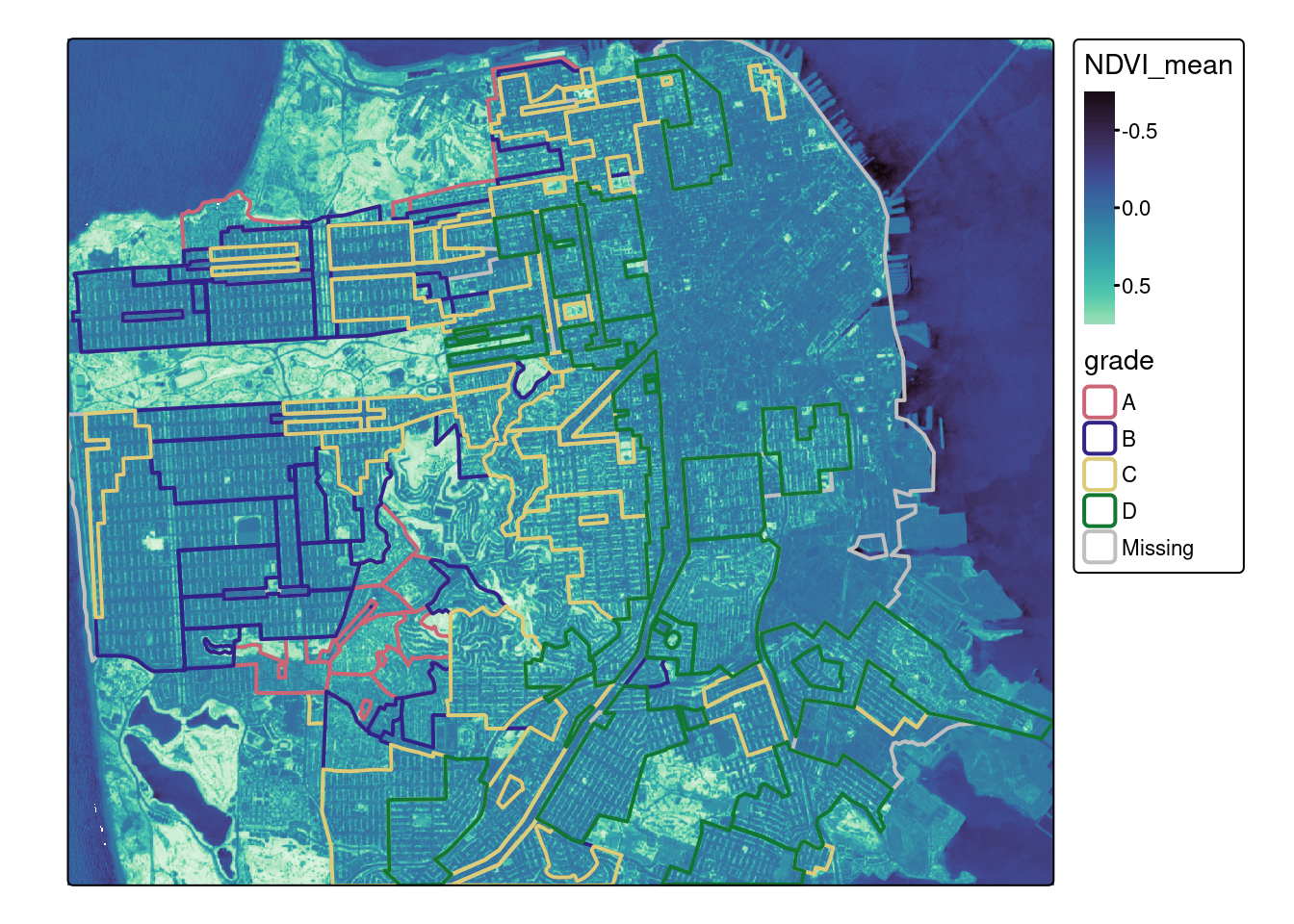

Interactive maps

tmap_mode("view")

tmap mode set to 'view'

tm_shape(ndvi_stars) + tm_raster(col.scale = mako) + 
  tm_shape(sf_redlines) + tm_borders("grade", lwd=2)